 mundialis GeoNetwork catalogue
GeoTIFF
Type of resources
Available actions
Topics
INSPIRE themes
Keywords
Contact for the resource
Provided by
Formats
Representation types
Update frequencies
status
Scale
Resolution
-
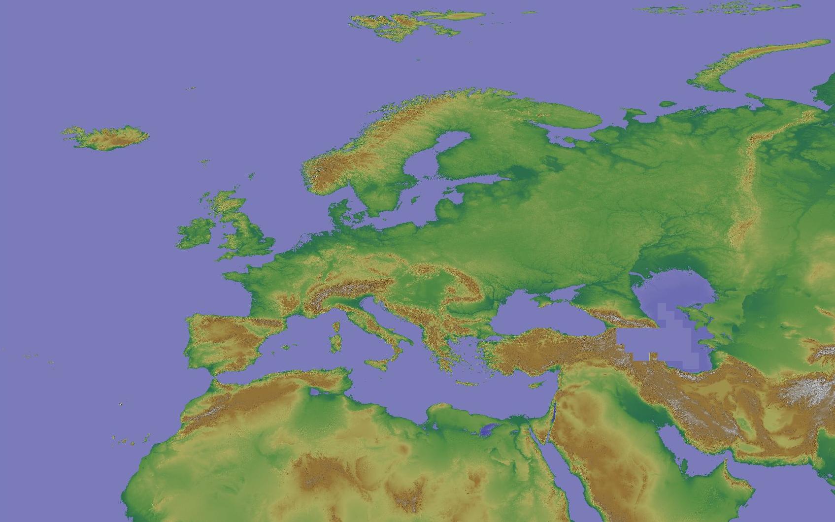
The Copernicus DEM is a Digital Surface Model (DSM) which represents the surface of the Earth including buildings, infrastructure and vegetation. The original GLO-30 provides worldwide coverage at 30 meters (refers to 10 arc seconds). Note that ocean areas do not have tiles, there one can assume height values equal to zero. Data is provided as Cloud Optimized GeoTIFFs. Note that the vertical unit for measurement of elevation height is meters. The Copernicus DEM for Europe at 3 arcsec (0:00:03 = 0.00083333333 ~ 90 meter) in COG format has been derived from the Copernicus DEM GLO-30, mirrored on Open Data on AWS, dataset managed by Sinergise (https://registry.opendata.aws/copernicus-dem/). Processing steps: The original Copernicus GLO-30 DEM contains a relevant percentage of tiles with non-square pixels. We created a mosaic map in https://gdal.org/drivers/raster/vrt.html format and defined within the VRT file the rule to apply cubic resampling while reading the data, i.e. importing them into GRASS GIS for further processing. We chose cubic instead of bilinear resampling since the height-width ratio of non-square pixels is up to 1:5. Hence, artefacts between adjacent tiles in rugged terrain could be minimized: gdalbuildvrt -input_file_list list_geotiffs_MOOD.csv -r cubic -tr 0.000277777777777778 0.000277777777777778 Copernicus_DSM_30m_MOOD.vrt In order to reduce the spatial resolution to 3 arc seconds, weighted resampling was performed in GRASS GIS (using r.resamp.stats -w) and the pixel values were scaled with 1000 (storing the pixels as integer values) for data volume reduction. In addition, a hillshade raster map was derived from the resampled elevation map (using r.relief, GRASS GIS). Eventually, we exported the elevation and hillshade raster maps in Cloud Optimized GeoTIFF (COG) format, along with SLD and QML style files.
-
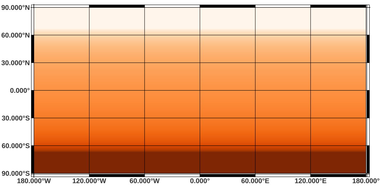
Overview: Daily maps for global daylight length, calculated for the year 2022. Processing steps: For each day within the year 2022, the photoperiod (sunshine hours on flat terrain) are calculated using the SOLPOS algorithm developed by the National Renewable Energy Laboratory (NREL), USA. Resultant values have been converted from hours to minutes. File naming scheme (DDD = day within year) (min is abbreviation for minute): daylight_min_2022_DDD.tif Projection + EPSG code: Latitude-Longitude/WGS84 (EPSG: 4326) Spatial extent: north: 90 south: -90 west: -180 east: 180 Spatial resolution: 30 arc seconds (approx. 1000 m) Temporal resolution: Daily Pixel values: unit: minutes Software used: GDAL 3.2.2 and GRASS GIS 8.2.0 Processed by: mundialis GmbH & Co. KG, Germany (https://www.mundialis.de/) Reference: National Renewable Energy Laboratory (NREL): SOLPOS 2.0 sun position algorithm (https://www.nrel.gov/grid/solar-resource/solpos.html)
-

Overview: ERA5-Land is a reanalysis dataset providing a consistent view of the evolution of land variables over several decades at an enhanced resolution compared to ERA5. ERA5-Land has been produced by replaying the land component of the ECMWF ERA5 climate reanalysis. Reanalysis combines model data with observations from across the world into a globally complete and consistent dataset using the laws of physics. Reanalysis produces data that goes several decades back in time, providing an accurate description of the climate of the past. Processing steps: The original hourly ERA5-Land air temperature 2 m above ground and dewpoint temperature 2 m data has been spatially enhanced from 0.1 degree to 30 arc seconds (approx. 1000 m) spatial resolution by image fusion with CHELSA data (V1.2) (https://chelsa-climate.org/). For each day we used the corresponding monthly long-term average of CHELSA. The aim was to use the fine spatial detail of CHELSA and at the same time preserve the general regional pattern and fine temporal detail of ERA5-Land. The steps included aggregation and enhancement, specifically: 1. spatially aggregate CHELSA to the resolution of ERA5-Land 2. calculate difference of ERA5-Land - aggregated CHELSA 3. interpolate differences with a Gaussian filter to 30 arc seconds. 4. add the interpolated differences to CHELSA Subsequently, the temperature time series have been aggregated on a daily basis. From these, daily relative humidity has been calculated for the time period 01/2000 - 07/2021. Relative humidity (rh2m) has been calculated from air temperature 2 m above ground (Ta) and dewpoint temperature 2 m above ground (Td) using the formula for saturated water pressure from Wright (1997): maximum water pressure = 611.21 * exp(17.502 * Ta / (240.97 + Ta)) actual water pressure = 611.21 * exp(17.502 * Td / (240.97 + Td)) relative humidity = actual water pressure / maximum water pressure Data provided is the daily averages of relative humidity. This set provides data for the years 2000 - 2004. For other time periods, please see further linked data sets. Resultant values have been converted to represent percent * 10, thus covering a theoretical range of [0, 1000]. File naming scheme (YYYY = year; MM = month; DD = day): ERA5_land_rh2m_avg_daily_YYYYMMDD.tif Projection + EPSG code: Latitude-Longitude/WGS84 (EPSG: 4326) Spatial extent: north: 82:00:30N south: 18N west: 32:00:30W east: 70E Spatial resolution: 30 arc seconds (approx. 1000 m) Temporal resolution: Daily Pixel values: Percent * 10 (scaled to Integer; example: value 738 = 73.8 %) Software used: GDAL 3.2.2 and GRASS GIS 8.0.0 Original ERA5-Land dataset license: https://apps.ecmwf.int/datasets/licences/copernicus/ CHELSA climatologies (V1.2): Data used: Karger D.N., Conrad, O., Böhner, J., Kawohl, T., Kreft, H., Soria-Auza, R.W., Zimmermann, N.E, Linder, H.P., Kessler, M. (2018): Data from: Climatologies at high resolution for the earth's land surface areas. Dryad digital repository. http://dx.doi.org/doi:10.5061/dryad.kd1d4 Original peer-reviewed publication: Karger, D.N., Conrad, O., Böhner, J., Kawohl, T., Kreft, H., Soria-Auza, R.W., Zimmermann, N.E., Linder, P., Kessler, M. (2017): Climatologies at high resolution for the Earth land surface areas. Scientific Data. 4 170122. https://doi.org/10.1038/sdata.2017.122 Processed by: mundialis GmbH & Co. KG, Germany (https://www.mundialis.de/) Reference: Wright, J.M. (1997): Federal meteorological handbook no. 3 (FCM-H3-1997). Office of Federal Coordinator for Meteorological Services and Supporting Research. Washington, DC Acknowledgements: This study was partially funded by EU grant 874850 MOOD. The contents of this publication are the sole responsibility of the authors and don't necessarily reflect the views of the European Commission.
-
Overview: ERA5-Land is a reanalysis dataset providing a consistent view of the evolution of land variables over several decades at an enhanced resolution compared to ERA5. ERA5-Land has been produced by replaying the land component of the ECMWF ERA5 climate reanalysis. Reanalysis combines model data with observations from across the world into a globally complete and consistent dataset using the laws of physics. Reanalysis produces data that goes several decades back in time, providing an accurate description of the climate of the past. Processing steps: The original hourly ERA5-Land air temperature 2 m above ground and dewpoint temperature 2 m data has been spatially enhanced from 0.1 degree to 30 arc seconds (approx. 1000 m) spatial resolution by image fusion with CHELSA data (V1.2) (https://chelsa-climate.org/). For each day we used the corresponding monthly long-term average of CHELSA. The aim was to use the fine spatial detail of CHELSA and at the same time preserve the general regional pattern and fine temporal detail of ERA5-Land. The steps included aggregation and enhancement, specifically: 1. spatially aggregate CHELSA to the resolution of ERA5-Land 2. calculate difference of ERA5-Land - aggregated CHELSA 3. interpolate differences with a Gaussian filter to 30 arc seconds. 4. add the interpolated differences to CHELSA Subsequently, the temperature time series have been aggregated on a daily basis. From these, daily relative humidity has been calculated for the time period 01/2000 - 07/2021. Relative humidity (rh2m) has been calculated from air temperature 2 m above ground (Ta) and dewpoint temperature 2 m above ground (Td) using the formula for saturated water pressure from Wright (1997): maximum water pressure = 611.21 * exp(17.502 * Ta / (240.97 + Ta)) actual water pressure = 611.21 * exp(17.502 * Td / (240.97 + Td)) relative humidity = actual water pressure / maximum water pressure The resulting relative humidity has been aggregated to decadal averages. Each month is divided into three decades: the first decade of a month covers days 1-10, the second decade covers days 11-20, and the third decade covers days 21-last day of the month. Resultant values have been converted to represent percent * 10, thus covering a theoretical range of [0, 1000]. The data have been reprojected to EU LAEA. File naming scheme (YYYY = year; MM = month; dD = number of decade): ERA5_land_rh2m_avg_decadal_YYYY_MM_dD.tif Projection + EPSG code: EU LAEA (EPSG: 3035) Spatial extent: north: 6874000 south: -485000 west: 869000 east: 8712000 Spatial resolution: 1000 m Temporal resolution: Decadal Pixel values: Percent * 10 (scaled to Integer; example: value 738 = 73.8 %) Software used: GDAL 3.2.2 and GRASS GIS 8.0.0 Original ERA5-Land dataset license: https://apps.ecmwf.int/datasets/licences/copernicus/ CHELSA climatologies (V1.2): Data used: Karger D.N., Conrad, O., Böhner, J., Kawohl, T., Kreft, H., Soria-Auza, R.W., Zimmermann, N.E, Linder, H.P., Kessler, M. (2018): Data from: Climatologies at high resolution for the earth's land surface areas. Dryad digital repository. http://dx.doi.org/doi:10.5061/dryad.kd1d4 Original peer-reviewed publication: Karger, D.N., Conrad, O., Böhner, J., Kawohl, T., Kreft, H., Soria-Auza, R.W., Zimmermann, N.E., Linder, P., Kessler, M. (2017): Climatologies at high resolution for the Earth land surface areas. Scientific Data. 4 170122. https://doi.org/10.1038/sdata.2017.122 Processed by: mundialis GmbH & Co. KG, Germany (https://www.mundialis.de/) Reference: Wright, J.M. (1997): Federal meteorological handbook no. 3 (FCM-H3-1997). Office of Federal Coordinator for Meteorological Services and Supporting Research. Washington, DC Acknowledgements: This study was partially funded by EU grant 874850 MOOD. The contents of this publication are the sole responsibility of the authors and don't necessarily reflect the views of the European Commission.
-
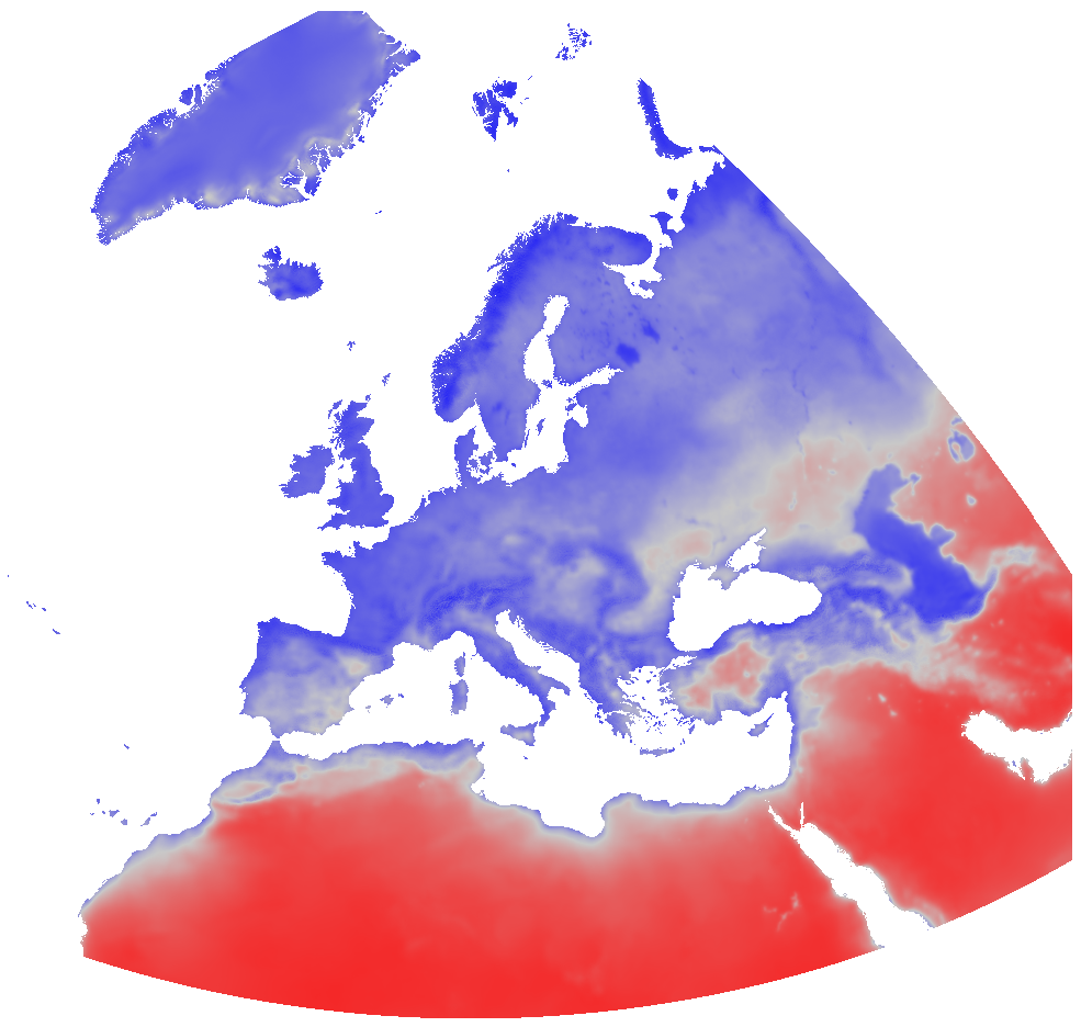
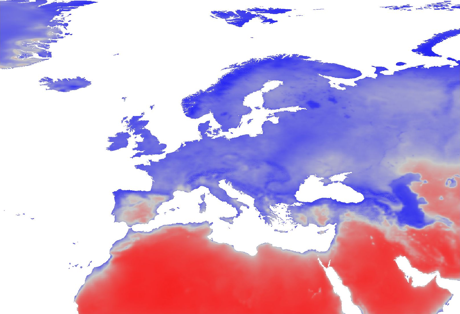
Overview: ERA5-Land is a reanalysis dataset providing a consistent view of the evolution of land variables over several decades at an enhanced resolution compared to ERA5. ERA5-Land has been produced by replaying the land component of the ECMWF ERA5 climate reanalysis. Reanalysis combines model data with observations from across the world into a globally complete and consistent dataset using the laws of physics. Reanalysis produces data that goes several decades back in time, providing an accurate description of the climate of the past. Air temperature (2 m): Temperature of air at 2m above the surface of land, sea or in-land waters. 2m temperature is calculated by interpolating between the lowest model level and the Earth's surface, taking account of the atmospheric conditions. Processing steps: The original hourly ERA5-Land data has been spatially enhanced from 0.1 degree to 30 arc seconds (approx. 1000 m) spatial resolution by image fusion with CHELSA data (V1.2) (https://chelsa-climate.org/). For each day we used the corresponding monthly long-term average of CHELSA. The aim was to use the fine spatial detail of CHELSA and at the same time preserve the general regional pattern and fine temporal detail of ERA5-Land. The steps included aggregation and enhancement, specifically: 1. spatially aggregate CHELSA to the resolution of ERA5-Land 2. calculate difference of ERA5-Land - aggregated CHELSA 3. interpolate differences with a Gaussian filter to 30 arc seconds 4. add the interpolated differences to CHELSA The spatially enhanced daily ERA5-Land data has been aggregated on a weekly basis starting from Saturday for the time period 2016 - 2020. Data available is the weekly average of daily averages, the weekly minimum of daily minima and the weekly maximum of daily maxima of air temperature (2 m). File naming: Average of daily average: era5_land_t2m_avg_weekly_YYYY_MM_DD.tif Max of daily max: era5_land_t2m_max_weekly_YYYY_MM_DD.tif Min of daily min: era5_land_t2m_min_weekly_YYYY_MM_DD.tif The date in the file name determines the start day of the week (Saturday). Pixel value: °C * 10 Example: Value 44 = 4.4 °C The QML or SLD style files can be used for visualization of the temperature layers. Coordinate reference system: ETRS89 / LAEA Europe (EPSG:3035) (EPSG:3035) Spatial extent: north: 82:00:30N south: 18N west: 32:00:30W east: 70E Spatial resolution: 1km Temporal resolution: weekly Time period: 01/01/2016 - 12/31/2020 Format: GeoTIFF Representation type: Grid Software used: GDAL 3.2.2 and GRASS GIS 8.0.0 (r.resamp.stats -w; r.relief) Lineage: Dataset has been processed from original Copernicus Climate Data Store (ERA5-Land) data sources. As auxiliary data CHELSA climate data has been used. Original ERA5-Land dataset license: https://cds.climate.copernicus.eu/api/v2/terms/static/licence-to-use-copernicus-products.pdf CHELSA climatologies (V1.2): Data used: Karger D.N., Conrad, O., Böhner, J., Kawohl, T., Kreft, H., Soria-Auza, R.W., Zimmermann, N.E, Linder, H.P., Kessler, M. (2018): Data from: Climatologies at high resolution for the earth's land surface areas. Dryad digital repository. http://dx.doi.org/doi:10.5061/dryad.kd1d4 Original peer-reviewed publication: Karger, D.N., Conrad, O., Böhner, J., Kawohl, T., Kreft, H., Soria-Auza, R.W., Zimmermann, N.E., Linder, P., Kessler, M. (2017): Climatologies at high resolution for the Earth land surface areas. Scientific Data. 4 170122. https://doi.org/10.1038/sdata.2017.122 Other resources: https://data.mundialis.de/geonetwork/srv/eng/catalog.search#/metadata/601ea08c-0768-4af3-a8fa-7da25fb9125b Processed by: mundialis GmbH & Co. KG, Germany (https://www.mundialis.de/) Contact: mundialis GmbH & Co. KG, info@mundialis.de Acknowledgements: This study was partially funded by EU grant 874850 MOOD. The contents of this publication are the sole responsibility of the authors and don't necessarily reflect the views of the European Commission.
-
Overview: ERA5-Land is a reanalysis dataset providing a consistent view of the evolution of land variables over several decades at an enhanced resolution compared to ERA5. ERA5-Land has been produced by replaying the land component of the ECMWF ERA5 climate reanalysis. Reanalysis combines model data with observations from across the world into a globally complete and consistent dataset using the laws of physics. Reanalysis produces data that goes several decades back in time, providing an accurate description of the climate of the past. Processing steps: The original hourly ERA5-Land air temperature 2 m above ground and dewpoint temperature 2 m data has been spatially enhanced from 0.1 degree to 30 arc seconds (approx. 1000 m) spatial resolution by image fusion with CHELSA data (V1.2) (https://chelsa-climate.org/). For each day we used the corresponding monthly long-term average of CHELSA. The aim was to use the fine spatial detail of CHELSA and at the same time preserve the general regional pattern and fine temporal detail of ERA5-Land. The steps included aggregation and enhancement, specifically: 1. spatially aggregate CHELSA to the resolution of ERA5-Land 2. calculate difference of ERA5-Land - aggregated CHELSA 3. interpolate differences with a Gaussian filter to 30 arc seconds. 4. add the interpolated differences to CHELSA Subsequently, the temperature time series have been aggregated on a daily basis. From these, daily relative humidity has been calculated for the time period 01/2000 - 07/2021. Relative humidity (rh2m) has been calculated from air temperature 2 m above ground (Ta) and dewpoint temperature 2 m above ground (Td) using the formula for saturated water pressure from Wright (1997): maximum water pressure = 611.21 * exp(17.502 * Ta / (240.97 + Ta)) actual water pressure = 611.21 * exp(17.502 * Td / (240.97 + Td)) relative humidity = actual water pressure / maximum water pressure The resulting relative humidity has been aggregated to decadal averages. Each month is divided into three decades: the first decade of a month covers days 1-10, the second decade covers days 11-20, and the third decade covers days 21-last day of the month. Resultant values have been converted to represent percent * 10, thus covering a theoretical range of [0, 1000]. File naming scheme (YYYY = year; MM = month; dD = number of decade): ERA5_land_rh2m_avg_decadal_YYYY_MM_dD.tif Projection + EPSG code: Latitude-Longitude/WGS84 (EPSG: 4326) Spatial extent: north: 82:00:30N south: 18N west: 32:00:30W east: 70E Spatial resolution: 30 arc seconds (approx. 1000 m) Temporal resolution: Decadal Pixel values: Percent * 10 (scaled to Integer; example: value 738 = 73.8 %) Software used: GDAL 3.2.2 and GRASS GIS 8.0.0 Original ERA5-Land dataset license: https://apps.ecmwf.int/datasets/licences/copernicus/ CHELSA climatologies (V1.2): Data used: Karger D.N., Conrad, O., Böhner, J., Kawohl, T., Kreft, H., Soria-Auza, R.W., Zimmermann, N.E, Linder, H.P., Kessler, M. (2018): Data from: Climatologies at high resolution for the earth's land surface areas. Dryad digital repository. http://dx.doi.org/doi:10.5061/dryad.kd1d4 Original peer-reviewed publication: Karger, D.N., Conrad, O., Böhner, J., Kawohl, T., Kreft, H., Soria-Auza, R.W., Zimmermann, N.E., Linder, P., Kessler, M. (2017): Climatologies at high resolution for the Earth land surface areas. Scientific Data. 4 170122. https://doi.org/10.1038/sdata.2017.122 Processed by: mundialis GmbH & Co. KG, Germany (https://www.mundialis.de/) Reference: Wright, J.M. (1997): Federal meteorological handbook no. 3 (FCM-H3-1997). Office of Federal Coordinator for Meteorological Services and Supporting Research. Washington, DC Acknowledgements: This study was partially funded by EU grant 874850 MOOD. The contents of this publication are the sole responsibility of the authors and don't necessarily reflect the views of the European Commission.
-
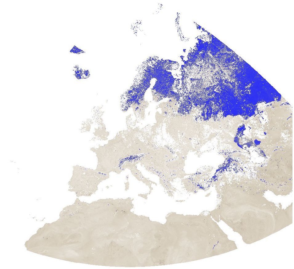
Modified Normalized Difference Water Index (MNDWI) from MODIS data for Europe at 1 km resolution. Source data: - MODIS/Terra Surface Reflectance 8-Day L3 Global 500 m SIN Grid (MOD09A1 v006): https://lpdaac.usgs.gov/products/mod09a1v006/ The corresponding MODIS/Aqua product (MYD09A1 v006) could not be used due to the fact that the Aqua satellite has a number of broken detectors resulting in unreliable data for band 6 (SWIR) measurements. The Moderate Resolution Imaging Spectroradiometer (MODIS) Terra MOD09A1 Version 6 product provides an estimate of the surface spectral reflectance of Terra MODIS Bands 1 through 7 corrected for atmospheric conditions such as gasses, aerosols, and Rayleigh scattering. Along with the seven 500 meter (m) reflectance bands are two quality layers and four observation bands. For each pixel, a value is selected from all the acquisitions within the 8-day composite period. The criteria for the pixel choice include cloud and solar zenith. When several acquisitions meet the criteria the pixel with the minimum channel 3 (blue) value is used. For the time periods October 2016 - March 2017 and August 2020 - April 2021, the original data has been reprojected to ETRS89-extended / LAEA Europe and aggregated to a 1 km grid. The temporal resolution is 8 days. Bad quality pixels (cloud, cloud shadow, dead detector, solar zenith angle too large, etc.) have been masked using the provided quality assurance (QA) layers and appear as "no data". File naming: productCode.acquisitionDate[A (YYYYDDD)]_mosaic_spatialResolution_frequency_VI.tif example: MOD09A1.A2016353_mosaic_1000m_8_days_MNDWI.tif The date is Year and Day of Year. Values are MNDWI * 10000. Example: Value -5099 = -0.5099
-

Temperature time series with high spatial and temporal resolutions are important for several applications. The new MODIS Land Surface Temperature (LST) collection 6 provides numerous improvements compared to collection 5. However, being remotely sensed data in the thermal range, LST shows gaps in cloud-covered areas. With a novel method [1] we fully reconstructed the daily global MODIS LST products MOD11C1 and MYD11C1 (spatial resolution: 3 arc-min, i.e. approximately 5.6 km at the equator). For this, we combined temporal and spatial interpolation, using emissivity and elevation as covariates for the spatial interpolation. Here we provide a time series of these reconstructed LST data aggregated as monthly average, minimum and maximum LST maps. [1] Metz M., Andreo V., Neteler M. (2017): A new fully gap-free time series of Land Surface Temperature from MODIS LST data. Remote Sensing, 9(12):1333. DOI: http://dx.doi.org/10.3390/rs9121333 The data available here for download are the reconstructed global MODIS LST products MOD11C1/MYD11C1 at a spatial resolution of 3 arc-min (approximately 5.6 km at the equator; see https://lpdaac.usgs.gov/dataset_discovery/modis/modis_products_table), aggregated to monthly data. The data are provided in GeoTIFF format. The Coordinate Reference System (CRS) is identical to the MOD11C1/MYD11C1 product as provided by NASA. In WKT as reported by GDAL: GEOGCS["Unknown datum based upon the Clarke 1866 ellipsoid", DATUM["Not specified (based on Clarke 1866 spheroid)", SPHEROID["Clarke 1866",6378206.4,294.9786982138982, AUTHORITY["EPSG","7008"]]], PRIMEM["Greenwich",0], UNIT["degree",0.0174532925199433]] Acknowledgments: We are grateful to the NASA Land Processes Distributed Active Archive Center (LP DAAC) for making the MODIS LST data available. The dataset is based on MODIS Collection V006. File name abbreviations: avg = average of daily averages min = minimum of daily minima max = maximum of daily maxima Meaning of pixel values: The pixel values are coded in degree Celsius * 100 (hence, to obtain °C divide the pixel values by 100.0).
-
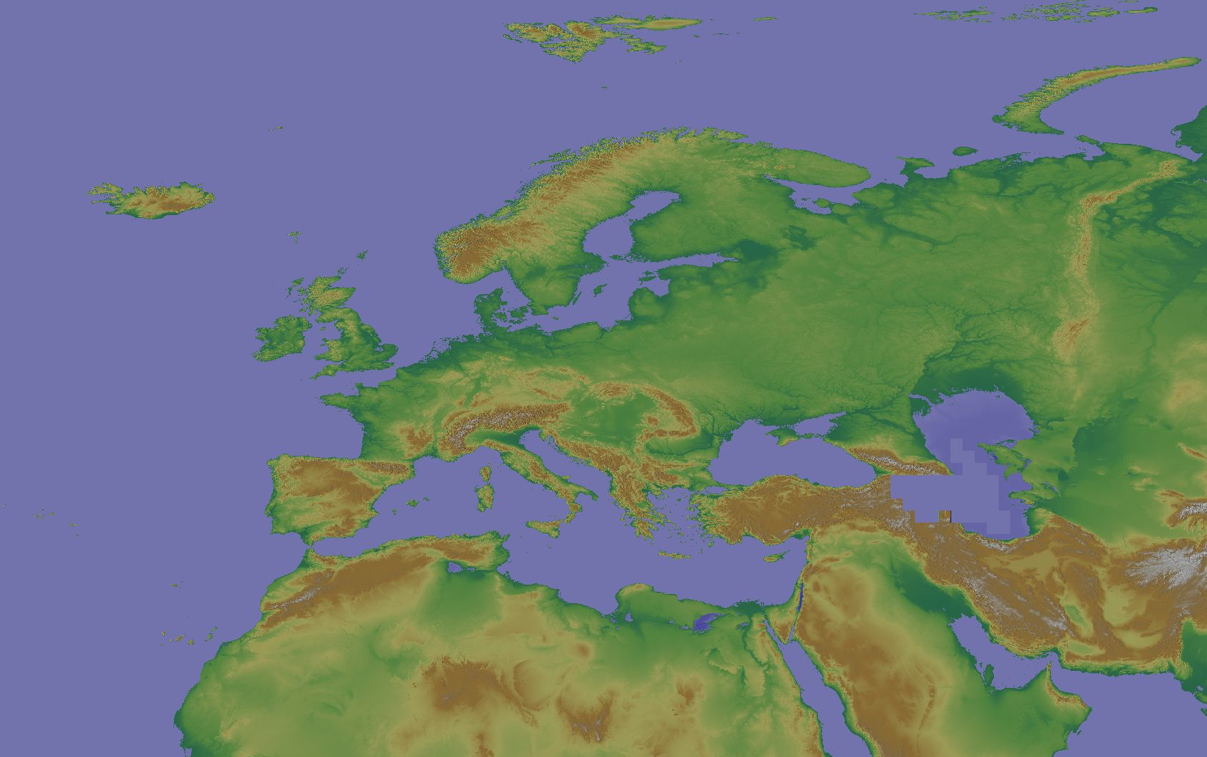
The Copernicus DEM is a Digital Surface Model (DSM) which represents the surface of the Earth including buildings, infrastructure and vegetation. The original GLO-30 provides worldwide coverage at 30 meters (refers to 10 arc seconds). Note that ocean areas do not have tiles, there one can assume height values equal to zero. Data is provided as Cloud Optimized GeoTIFFs. Note that the vertical unit for measurement of elevation height is meters. The Copernicus DEM for Europe at 30 arcsec (0:00:30 = 0.0083333333 ~ 1000 meter) in COG format has been derived from the Copernicus DEM GLO-30, mirrored on Open Data on AWS, dataset managed by Sinergise (https://registry.opendata.aws/copernicus-dem/). Processing steps: The original Copernicus GLO-30 DEM contains a relevant percentage of tiles with non-square pixels. We created a mosaic map in a https://gdal.org/drivers/raster/vrt.html format and defined within the VRT file the rule to apply cubic resampling while reading the data, i.e. importing them into GRASS GIS for further processing. We chose cubic instead of bilinear resampling since the height-width ratio of non-square pixels is up to 1:5. Hence, artefacts between adjacent tiles in rugged terrain could be minimized: gdalbuildvrt -input_file_list list_geotiffs_MOOD.csv -r cubic -tr 0.000277777777777778 0.000277777777777778 Copernicus_DSM_30m_MOOD.vrt In order to reduce the spatial resolution to 30 arc seconds, weighted resampling was performed in GRASS GIS (using r.resamp.stats) and the pixel values were scaled with 1000 (storing the pixels as integer values) for data volume reduction. In addition, a hillshade raster map was derived from the resampled elevation map (using r.relief, GRASS GIS). Eventually, we exported the elevation and hillshade raster maps in Cloud Optimized GeoTIFF (COG) format, along with SLD and QML style files.
-
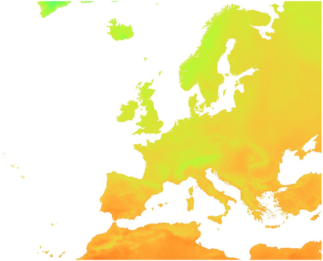
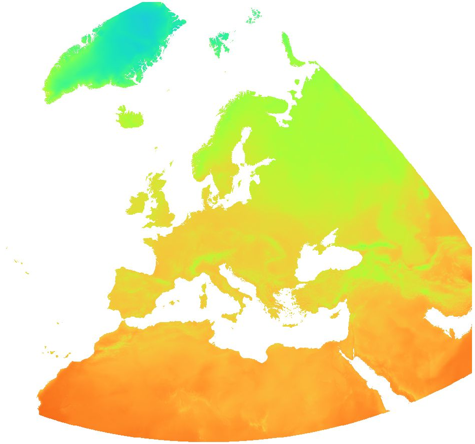
Overview: ERA5-Land is a reanalysis dataset providing a consistent view of the evolution of land variables over several decades at an enhanced resolution compared to ERA5. ERA5-Land has been produced by replaying the land component of the ECMWF ERA5 climate reanalysis. Reanalysis combines model data with observations from across the world into a globally complete and consistent dataset using the laws of physics. Reanalysis produces data that goes several decades back in time, providing an accurate description of the climate of the past. Surface temperature: Temperature of the surface of the Earth. The skin temperature is the theoretical temperature that is required to satisfy the surface energy balance. It represents the temperature of the uppermost surface layer, which has no heat capacity and so can respond instantaneously to changes in surface fluxes. The original ERA5-Land dataset (period: 2000 - 2020) has been reprocessed to: - aggregate ERA5-Land hourly data to daily data (minimum, mean, maximum) - while increasing the spatial resolution from the native ERA5-Land resolution of 0.1 degree (~ 9 km) to 30 arc-sec (~ 1 km) by image fusion with CHELSA data (V1.2) (https://chelsa-climate.org/). For each day we used the corresponding monthly long-term average of CHELSA. The aim was to use the fine spatial detail of CHELSA and at the same time preserve the general regional pattern and fine temporal detail of ERA5-Land. The steps included aggregation and enhancement, specifically: 1. spatially aggregate CHELSA to the resolution of ERA5-Land 2. calculate difference of ERA5-Land - aggregated CHELSA 3. interpolate differences with a Gaussian filter to 30 arc seconds 4. add the interpolated differences to CHELSA Data available is the daily average, minimum and maximum of surface temperature. Software used: GDAL 3.2.2 and GRASS GIS 8.0.0 (r.resamp.stats -w; r.relief) Original ERA5-Land dataset license: https://cds.climate.copernicus.eu/api/v2/terms/static/licence-to-use-copernicus-products.pdf CHELSA climatologies (V1.2): Data used: Karger D.N., Conrad, O., Böhner, J., Kawohl, T., Kreft, H., Soria-Auza, R.W., Zimmermann, N.E, Linder, H.P., Kessler, M. (2018): Data from: Climatologies at high resolution for the earth's land surface areas. Dryad digital repository. http://dx.doi.org/doi:10.5061/dryad.kd1d4 Original peer-reviewed publication: Karger, D.N., Conrad, O., Böhner, J., Kawohl, T., Kreft, H., Soria-Auza, R.W., Zimmermann, N.E., Linder, P., Kessler, M. (2017): Climatologies at high resolution for the Earth land surface areas. Scientific Data. 4 170122. https://doi.org/10.1038/sdata.2017.122